Sampling
How Well Does a Sample Describe the Population?
All files, sofware, and tutorials that make up SABLE Copyright (c) 1997 1998
1999 Virginia Tech. You may use these programs under the conditions of the
SABLE General License, which
incorporates the
GNU GENERAL PUBLIC LICENSE.
Introduction
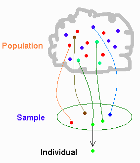
A sample is a collection of individuals selected from a larger population.
For example, we may have a single sample composed of 50 cases, representing
a population of 1000 individuals. Sometimes in everyday language we use
the word "sample" to refer to a specific individual.
Here we will use "sample" to mean a collection of individuals. This tutorial
explains how the size of the sample and the procedure used to select the
sample affect how well the sample reflects the population.

How Can Samples Reveal Information About Individuals Not Included in the
Sample?
Social scientists collect samples when the population is too large, or
too dynamic, to permit examination of every individual. If a sample has
been collected properly, we can make useful inferences about characteristics
of the parent population, such as the mean value for some variable. Samples
do not inform us about exact characteristics of populations, but instead
provide estimates or approximations.
1. Approximating
the Population Mean.
You will be given a "population" of circles whose mean (average)
radius will be shown in the panel below the circles. Click on circles
to collect a small sample whose mean radius is close to the population
mean. The mean of your sample will also be displayed below the
circles. Compare your sample mean to the population mean, and select
larger or smaller circles to bring your sample mean within the target
range.
Once you reach your target, the results are displayed, and
then the exercise will repeat with a new target that is closer to the
population mean.
Try to keep your samples as small as possible. Notice what
happens to your sample size as the target approaches the true
mean. You will probably have to choose circles carefully to avoid
including the entire population in your sample.
You can see from this activity that it is possible for a sample of
circles to provide information about all the circles in the
population, even though only a few are included
in the sample. With practice, you can select a small sample that
provides an estimate that is very close to the true value.
In general, however, creating a sample that is a better representation
of the entire population requires more individuals than creating a less
accurate representation.
Sample Characteristics
Social scientists do not select samples by deliberately choosing a "proper"
mix of individuals, as you were able to do in the previous activity. In fact,
good sampling
procedures require just the opposite:
They deliberately prevent investigators
from choosing specific individuals. The effectiveness of a sample is related
to the degree of randomness applied in selecting individuals. Samples
have power to the extent that they represent the population to be studied.
Representativeness can be relied upon only when samples are composed of
observations that have been selected without influence of the investigator.
We can refer to samples compiled at random as Random Samples,
meaning that individuals are selected from a population, so that each
member of the population has a known chance of selection for a sample.
There is an important distinction between an arbitrarily selected individual,
and one that is truly random. If we select an individual to become a member
of a sample haphazardly, without careful thought, we may meet an everyday
definition of randomness. But we may in fact be selecting only individuals
that are convenient to collect, or that meet an investigator's inaccurate
notion of what constitutes a "good" representative of the population.
In contrast, true randomness is assured when the sampling procedure
is carefully designed to remove any element of choice. Random samples are
collected according to a procedure (sometimes known as a protocol)
specifically tailored for the individual study, that gives precise steps
to assure that each individual in the population has a known chance of
selection. Usually such a procedure is based upon use of a table of random
numbers to select the sample.
2. The Sampler
Here is another population of circles, whose mean diameter is given. The
distribution of circle diameters is presented in a histogram (chart) as well.
Type a sample size in the text area and click the "Take a Sample" button.
A sample of that size will be randomly collected from the population. The
sample mean diameter will be displayed, and the distribution will be drawn on
top of the population histogram.
Experiment with sample sizes from very small to nearly all the population.
Notice how results vary when you use separate trials with a
constant sample size (click on "Take a Sample" several times without
changing the sample size). Observe that results
vary most noticeably when sample sizes are small.
Selecting a small sample size does not necessarily mean that the estimate will be
inaccurate, and similarly, choosing a larger sample size will not guarantee
accurate estimates. But, if (for example) we pick ten samples of 5 individuals
each, we will tend, on the average, to obtain less accurate estimates than
if we pick ten samples of 50 individuals each. Notice also that estimates
of the mean from a series of larger samples tend to vary less than do those
from a series of smaller samples.
You can prove these facts to yourself using the Sampler activity! Take ten
small samples and count how many times the sample mean was within 0.5 of the
population mean. Now do the same thing for a larger sample. How small a sample
can you use and still have your sample mean in this range 80% of the time? (Results
will vary.)
Central Limit Theorem
How likely a particular size sample accurately estimates the
population characteristics is an important topic to researchers.
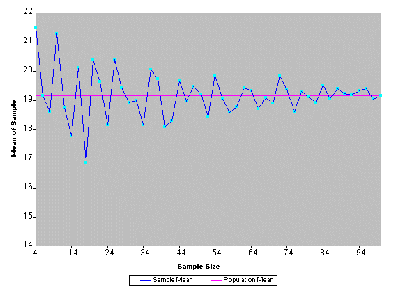
Below is a graph of results from the Sampler activity. Samples were taken at
increasing sizes, from 4 cases to 98 cases. You can see that as sample size increases,
not only do the sample means become closer to the population
mean, but fluctuations in sample means becomes smaller.
 There is a wide variation in results of small samples. Suppose you
were trying to determine the average height of students in your
school. If you collect information from five people, you may or may
not have a good estimate. If you sampled another five people, you
probably would not come up with the same estimate. If you take this
small sample over and over, you would get a lot of different sample
means. In contrast, suppose you were able to sample the entire
population. No matter how many times you took your sample, it would
always have the same mean. It would of course be ridiculous to
repeatedly sample an unchanging population. But this illustrates that,
as sample size increases, the frequency of samples having means equal
or close to the population characteristic increases.
3. Means of Repeated Samples
In the following activity, type in a value for "sample size"
and then click the "Get Samples" button.
You will see a frequency histogram of the means of 200 different samples
of that size. Start with a small sample size, like 10, and work up to larger
samples. Notice how the histogram shows fewer different values for means
of larger sample sizes, indicating that these means tend to converge to the
population mean.
This activity illustrates the effect of choosing specific sample sizes.
Small sample sizes, such as 10 or 15 for example, have a mean that tends
to vary widely, as revealed by the wide range in the histogram of estimates.
Increasing the sample size to 50 or 60, for example, reduces the wide swings
in estimates of the overall mean.
Furthermore, as sample size increases, the shape of the histogram tends
to assume a more symmetric shape, with a single large value near the center
of the distribution and declining numbers on either side, taking a bell-shape
form as they decline to smaller frequencies.
This general shape, known as the normal frequency distribution,
is characteristic of data acquired by random sampling.
If we randomly select samples from populations, even populations with
non-normal distributions, the frequency distributions of sample means
will begin to approximate the normal frequency distribution as sample
size increases.
This important concept is known as the
Central Limit Theorem.
These results illustrate why increasing sample size is so valuable.
Randomness avoids introducing investigator bias. Random sampling
causes the means for a series of samples to approximate the normal frequency
distribution, which allows us to use other statistical tests to estimate
the reliability of samples. Large sample sizes minimize sampling
error, assuring that information from the sample is as accurate as possible.
Stratification
Often we focus our sampling effort on specific parts of a population. We
do this to acquire more specific information, and to make effective use
of the sampling effort. Stratification
means that the investigator has enough knowledge of the population to subdivide
the population, and to allocate sampling effort accordingly. For example,
an investigator interested in aging might stratify samples by age
to direct the sampling effort at the individuals of greatest interest to
the study. There are relatively few people over 80 years old. If the investigator
is especially interested in information about people over 80, more people
in this age group may need to be sampled than would occur if the entire
population were sampled at random.
Another useful application of stratified data is to make corrections to
account for groups known to be underrepresented in a set of data. For
example, about half the population are women. If your survey results include
only 25% women, you may want to use a higher fraction of the women's
responses to obtain a representation of men and women equal to that in
the population.
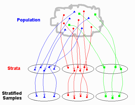
Within strata,
individuals are collected randomly.
In the following picture, the population has been divided into three
strata each of different size.
To get samples for each strata of the same size, the researcher must
sample a higher percentage of the population from the third strata.

We can also stratify data to detect similarities or differences across
different groups. We might want to answer questions such as:
-
Do older women tend to vote Republican more than younger women?
-
Is there a difference between attitudes of younger and older women on the
topic of abortion?
-
Is there a difference between rural and urban people in their support for
capital punishment?
4. Stratification
Choose a variable and stratification scheme and compare samples from different strata.
Answer questions in the panel on the right.
Stratifying allows us to compare different segments of a population, but
in these examples, we have not really discussed
how to decide if two samples are different. If 32%
of the women under 40 years of age vote Republican,
and 33% of the women over 40 vote Republican, then
it is reasonable to conclude that the 1%
difference does not signify a genuine difference between
the two groups.
It is more likely to result from the variance caused by a samll sample
size.
But what conclusion do we draw when the difference
is 2%? 3%? How large does the difference
have to become before we can be confident that we are
observing genuine differences between the two groups?
A large part of the field of statistics is devoted to
providing clear, systematic procedures for answering such
questions. In our system of tutorials, we introduce these
topics in Measures of Dispersion,
which is devoted to describing variation within samples, and
Hypothesis Testing,
which examines how to compare samples.
Summary
This tutorial has introduced some of the concepts important in planning
effective use of samples. We emphasize the advantages
of using large samples, which produce clear improvements in accuracy
and precision. You might conclude that large samples are always better
-- given these advantages, why would anyone ever use a small sample size?
Effort is required to collect every sample. The activities in
this tutorial do not show that costs in time and effort increase as a
researcher increases sample size. Thus, researchers have powerful
economic incentives to minimize the costs of sampling. The challenge
in designing a sampling plan is to strike an effective balance between
the statistical advantages of large sample sizes and the cost
advantages of small sample sizes.
Go to Top of Page
Return to Table
of Contents
Report Problems to SoSci
Updated June 23, 1998
